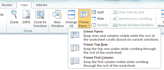
While working in excel sheets, we mostly label the columns of the top most row according to the content the column is going to contain. But after adding some rows of content, the top most row with the labels is scrolled away and we have to judge the label of the column by reading its content. But not now, we have a solution.
What Is Freezing Of Rows In Excel
Freezing is a way of keeping rows or columns visible at all times, even if you scroll down. With freezing rows in Excel, you can keep the topmost row, leftmost column, or any number or rows/columns within the excel sheet in view all the time.
Freeze Topmost Row And Left Most Column
Freezing the topmost row or the leftmost column in Microsoft Excel is dead simple. From the top navigation, go to View. Now under the Window group, select Freeze Panes. Now from the pop-up menu, select “Freeze Top Row” to freeze the top most row and “Freeze First Column” to freeze the leftmost column.

To freeze certain rows in Excel, first scroll to the first row to be frozen (the first row you want to freeze needs to be the first row visible on screen), now select all the rows you want to freeze and click the Freeze Panes button. Do the same if you wish to freeze certain columns.
If you want to unfreeze your rows and/or columns, select the Unfreeze Panes button. Unfreeze Panes button will appear in place of Freeze Panes button once you freeze any row/column.